Transformers are novel neural networks that are mainly used for sequence transduction tasks. Sequence transduction is any task where input sequences are transformed into output sequences. Most competitive neural sequence transduction models have an encoder-decoder structure. The encoder maps an input sequence of symbol representations to a sequence of continuous representations, the decoder then generates an output sequence of symbols one element at a time. At each step the model is auto-regressive, consuming the previously generated symbols as additional input when generating the next. In this post, I’ll document my learnings on main building blocks of transformer and how to implement them using PyTorch.
import copy
import torch
import math
import torch.nn as nn
from torch.nn.functional import log_softmax, pad

class EncoderDecoder(nn.Module):
    """
    A standard Encoder-Decoder architecture.
    """

    def __init__(self, encoder, decoder, src_embed, tgt_embed, generator):
        super(EncoderDecoder, self).__init__()
        self.encoder = encoder
        self.decoder = decoder
        self.src_embed = src_embed
        self.tgt_embed = tgt_embed
        self.generator = generator

    def forward(self, src, tgt, src_mask, tgt_mask):
        # Take in and process masked src and target sequences.
        return self.decode(self.encode(src, src_mask), src_mask, tgt, tgt_mask)

    def encode(self, src, src_mask):
        # Pass input sequence i.e. src through encoder
        return self.encoder(self.src_embed(src), src_mask)

    def decode(self, memory, src_mask, tgt, tgt_mask):
        # Memory is the query and key from encoder
        return self.decoder(self.tgt_embed(tgt), memory, src_mask, tgt_mask)


class Generator(nn.Module):
    # Define standard linear + softmax generation step.

    def __init__(self, d_model, vocab):
        super(Generator, self).__init__()
        self.proj = nn.Linear(d_model, vocab)

    def forward(self, x):
        return log_softmax(self.proj(x), dim=-1)
Encoder
Encoder’s job is to convert an input sequence of tokens into a contextualized sequence of embedding vectors. By contextualized we mean the embedding of each token contains information about the context of the sequence such that the word “apple” as a fruit have a different embedding than “apple” as a company.
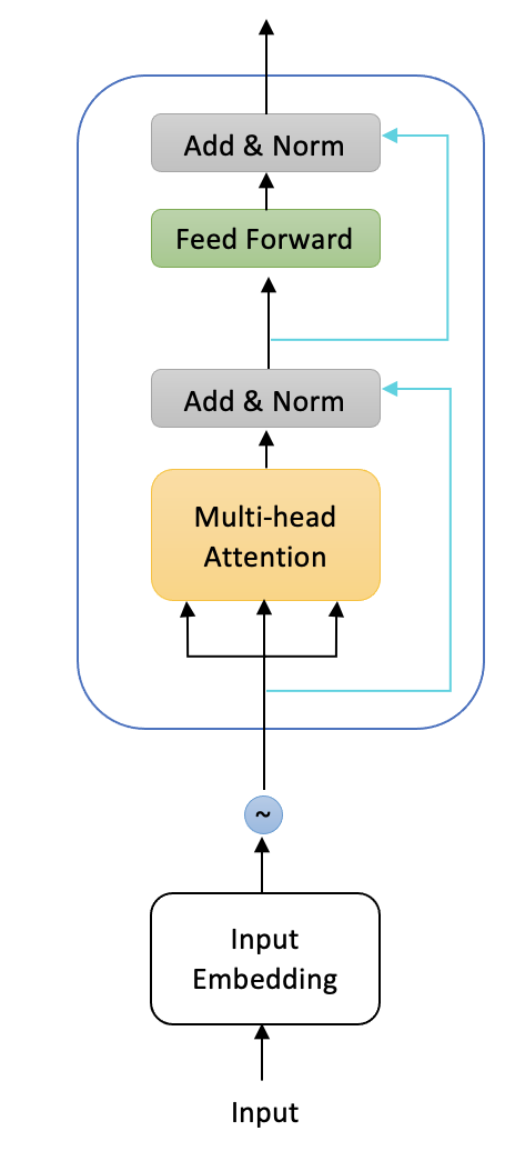
The encoder block is demonstrated in the figure below; it consists of multiple (historically 6) encoder layers. First encoder layer, takes the input embedding and add positional embeddings to it. Positional embeddings is shown as $\sim$ symbol in the image, and we’ll explain it soon. This only happens in the first encoder layer. All encoder layers has two sub-layers: a multi-head self-attention mechanism, and a simple, position-wise fully connected feed-forward network. Each encoder layer receives a sequence of embeddings and feeds them through the two sublayers. The output embedding of an encoder layer has the same size as its inputs, and it is passed to the next encoder layer. Eventually all encoder layers together update the input embeddings so that they contain some contextual information from the sequence.
Each encoder layer uses skip connections, shown with cyan arrows in the image below, and layer normalization, shows as “add & norm” box in the image below. Before, we dive into the encoder code, we explain each of these components.
 | Skip connection also known as residual connection pass a tensor to the next layer without processing and add it to the processed tensor. Skip connection is a simple yet very effective technique to mitigate the vanishing gradient problem in training deep neural networks and help them converge faster. They were first introduced in ResNet in computer vision.
|
Positional Embedding
In addition to embed semantic of a token, we need to embed token’s position in the sequence too. This is because transformer processes input tokens in parallel and not sequentially; as a result it does not carry any information on positions of tokens, so we need to embed this information into the input. Positional embeddings are identifiers that are added to tokens’ embeddings, and must satisfy two requirements:
- It should be the same for a position irrespective of the token in that position. So while the sequence might change, the positional embeddings must stay the same.
- They should not be too large, or otherwise they will dominate semantic similarity.
Based on above criteria, we can not use a non-periodic function (e.g. linear) that numbers tokens from 1 to total number of tokens. Such functions violate the second requirement above. A working option would be to use sine and cosine functions. Sine and cosine periodically return a number in $(-1,1)$ range and are bounded. They are defined everywhere, and so even on very large sequences all tokens receive a positional embedding. Moreover, they have large variability even for large numbers. This is in contrast to sigmoid function which gets flat on large values. The disadvantage of sine/cosine is that it repeats same outcome for many positions. This is not desirable, so we can give our function a low frequency (so that sine/cosine is stretched) such that even for our biggest sequence length the numbers do not repeat. This has the benefit of the linear function while positions are bounded BUT it has the cons of having little difference between consecutive positions. We want different positions to have meaningful differences. So we use a low-frequency sine for first dimension of positional embeddings. For the second dimension, we use cosine with a higher frequency.
We repeat this for all dimensions: alternate between sine and cosine and increase frequency. In math, $PE_{(pos, 2i)} = \sin(pos/10000^{2i/d_{model}})$ and $PE_{(pos, 2i+1)} = \cos(pos/10000^{2i/d_{model}})$ for position $pos$ and dimension $i$.
class PositionalEncoding(nn.Module):
    # Implement the position encoding (PE) function.

    def __init__(self, d_model, dropout, max_len=5000):
        super(PositionalEncoding, self).__init__()
        self.dropout = nn.Dropout(p=dropout)

        # Compute the positional encodings once in log space.
        pe = torch.zeros(max_len, d_model)
        position = torch.arange(0, max_len).unsqueeze(1)
        div_term = torch.exp(
            torch.arange(0, d_model, 2) * -(math.log(10000.0) / d_model)
        )
        pe[:, 0::2] = torch.sin(position * div_term)
        pe[:, 1::2] = torch.cos(position * div_term)
        pe = pe.unsqueeze(0)
        self.register_buffer("pe", pe)

    def forward(self, x):
        # adds token embedding to its position embedding
        x = x + self.pe[:, : x.size(1)].requires_grad_(False)
        return self.dropout(x)
P.s. This method works well for text. For images, people use relative positional embedding. Frequency is a different way of measuring horizontal stretch. With sinusoidal functions, frequency is the number of cycles that occur in $2\pi$. For example, frequency of $sin(3x)$ is $3$, and frequency of $\sin(x/3)$ is $1/3$.
Multi-head attention
The multi-head attention consists of multiple attention heads. Each attention head is a mechanism that assign a different amount of weight or “attention” to each element in the sequence. It does so by updating each token embedding as weighted average of all token embeddings in the sequence. Embeddings that are generated in this way are called contextualized embeddings. The weights in the weighted average are called attention weights. There are several ways to implement a self-attention layer; the most common method is scaled dot-product attention.
Scaled dot-product attention
There are three main steps in this method:
- First, It projects each token embedding into three vectors called query, key and value. It does so by applying three independent linear projections to each token embedding. If $T \in \mathbb{R}^d$ is the input token embedding in $d$ dimensional space, and $W^Q \in \mathbb{R}^k, W^K \in \mathbb{R}^k$ and $W^V \in \mathbb{R}^v$ denote projections matrices for computing query, key and value, then the respective embedding would be $Q = TW^Q, K=TW^K$ and $V=TW^V$.
- Second, computes attention scores. It measures similarity of a query and a key via dot-product method, which computes very efficiently using matrix multiplications. Queries and keys which are similar will have a very large dot-product, while those that don’t share much in common will have little to no overlap. The outcome of this step is called attention scores. For a sequence with $n$ input tokens, there is a corresponding $n\times n$ matrix of attention scores.
- Third it computes attention weights. Dot-products be arbitrary large and will lead to destabilizing training, therefore in this step we scale them down by dividing by $\sqrt{dim}$, and then apply softmax to make them sum up to $1$. If we don’t scale down by $\sqrt{dim}$ the softmax we apply might saturate early. The outcome of softmax is called attention weights.
- It then updates token embeddings as weighted average of value embeddings, where weights are the attention weights.

We will explain the Mask (optional) in later sections when we discuss decoder.
In code,
def attention(query, key, value, mask=None, dropout=None):
    '''
     Compute Scaled Dot Product Attention
    '''

    d_k = query.size(-1)
    scores = torch.matmul(query, key.transpose(-2, -1)) / math.sqrt(d_k)
    if mask is not None:
        scores = scores.masked_fill(mask == 0, -1e9)
    p_attn = scores.softmax(dim = -1)
    if dropout is not None:
        p_attn = dropout(p_attn)
    return torch.matmul(p_attn, value), p_attn
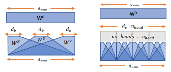
It is beneficial to have multiple attention head and combine their embeddings. Multi-head attention jointly attend to information from different representation subspaces by concatenating them and passing them through a linear projection. Figure below, shows single attention and multi-head attention where they receive token embeddings in $d_{model}$ dimension, and outputs contextualized embeddings in $d_{model}$ dimension. Note since $d_v$ does not need to be same as $d_{model}$, we pass it throuhg a final linear layer denoted as $W^0$ to project results back to $d_{model}$ dimension.
In code,
class MultiHeadedAttention(nn.Module):
    def __init__(self, h, d_model, dropout=0.1):
        # Take in model size and number of heads.

        super(MultiHeadedAttention, self).__init__()
        assert d_model % h == 0
        # We assume d_v always equals d_k
        self.d_k = d_model // h
        self.h = h
        self.linears = clones(nn.Linear(d_model, d_model), 4)
        self.attn = None
        self.dropout = nn.Dropout(p=dropout)

    def forward(self, query, key, value, mask=None):
        if mask is not None:
            # Same mask applied to all h heads.
            mask = mask.unsqueeze(1)
        nbatches = query.size(0)

        # Do all the linear projections in batch from d_model => h x d_k
        query, key, value = [
            lin(x).view(nbatches, -1, self.h, self.d_k).transpose(1, 2)
            for lin, x in zip(self.linears, (query, key, value))
        ]

        # Apply attention on all the projected vectors in batch.
        x, self.attn = attention(
            query, key, value, mask=mask, dropout=self.dropout
        )

        # Concat using a view and apply a final linear.
        x = (
            x.transpose(1, 2)
            .contiguous()
            .view(nbatches, -1, self.h * self.d_k)
        )
        return self.linears[-1](x)
Feed-Forward Layer
This sub-layer is just a simple two layer fully connected neural network that processes embedding vector independently. This is in contrast to processing the whole sequence of embeddings as a single vector. For this reason, this layer is often referred to as position-wise feed-forward layer. Usually the hidden size of the first layer is $4d_{model}$ and a GELU activation function is mostly used. This is where most of the memorization happens, and when scaling the model this dimension usually scales up.
Decoder
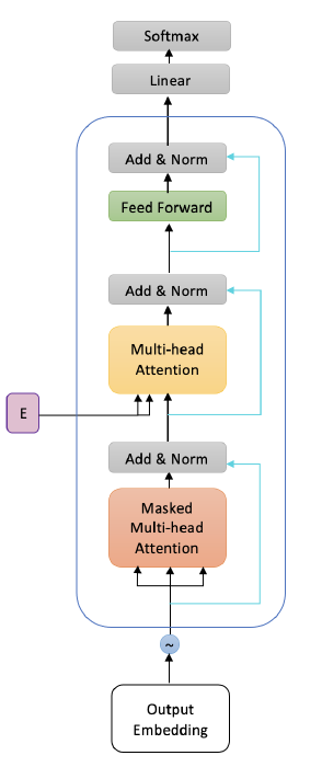
The decoder’s job is to generate text sequences. Below, we see an image of the decoder block, and as we see it consists of multiple decoder layers. Every decoder layer has two multi-headed attention sub-layers, a pointwise feed-forward layer, residual connections, and layer normalization. As we see, the decoder block is capped off with a linear layer that acts as a classifier, and a softmax to get the word probabilities. The decoder is autoregressive, it begins with a start token, and it takes in a list of previous outputs as inputs, as well as the encoder outputs that contain the attention information from the input. The decoder stops decoding when it generates a token as an output.
While feed-forward sub-layer behaves similarly as its counterpart in encoder, the two multi-headed attention (MHA) sub-layers are slightly different from MHA in encoder. Below, we explain the differences.
First masked multi-head attention: To prevent the decoder from looking at future tokens, a look ahead mask is applied. So the decoder is only allowed to attend to earlier positions in the output sequence. The mask is added before calculating the softmax, and after scaling the scores in attention mechanism. So it computes the scaled dot-product scores between query and keys, then adds the look-ahead mask to mask future words, then calculate softmax on them. The look-ahead mask is a key-by-key square matrix where lower diagonal of it is zero, and upper diagonal is set to $-\infty$. Once you take the softmax of the masked scores, the negative infinities get zeroed out, leaving zero attention scores for future tokens. This masking is the only difference in how the attention scores are calculated in the first multi-headed attention layer.
Second multi-head attention: For this layer, the encoder’s outputs are the queries and the keys, and the first multi-headed attention layer outputs are the values. This process matches the encoder’s input to the decoder’s input, allowing the decoder to decide which encoder input is relevant to put a focus on. The output of the second multi-headed attention goes through a pointwise feedforward layer for further processing.
def subsequent_mask(size):
    # Mask out subsequent positions.
    attn_shape = (1, size, size)
    subsequent_mask = torch.triu(torch.ones(attn_shape), diagonal=1).type(torch.uint8)
    return subsequent_mask == 0

class DecoderLayer(nn.Module):
    # Decoder is made of self-attn, src-attn, and feed forward (defined below)"

    def __init__(self, size, self_attn, src_attn, feed_forward, dropout):
        super(DecoderLayer, self).__init__()
        self.size = size
        self.self_attn = self_attn
        self.src_attn = src_attn
        self.feed_forward = feed_forward
        self.sublayer = clones(SublayerConnection(size, dropout), 3)

    def forward(self, x, memory, src_mask, tgt_mask):
        # Follow Figure 1 (right) for connections."
        m = memory
        x = self.sublayer[0](x, lambda x: self.self_attn(x, x, x, tgt_mask))
        x = self.sublayer[1](x, lambda x: self.src_attn(x, m, m, src_mask))
        return self.sublayer[2](x, self.feed_forward)


class Decoder(nn.Module):
    # Generic N layer decoder with masking."

    def __init__(self, layer, N):
        super(Decoder, self).__init__()
        self.layers = clones(layer, N)
        self.norm = LayerNorm(layer.size)

    def forward(self, x, memory, src_mask, tgt_mask):
        for layer in self.layers:
            x = layer(x, memory, src_mask, tgt_mask)
        return self.norm(x)
The full code is available at https://github.com/mina-ghashami/transformer-in-pytorch
Thank you
If you have any questions please reach out to me:
https://www.linkedin.com/in/minaghashami/
Follow me on medium for more content: https://medium.com/@mina.ghashami